线性回归模型是一个朴素而强大的工具,可以帮我们发现潜藏于数据下的规律,具体来讲,是因素如何影响目标变量的规律。
一元线性回归模型#
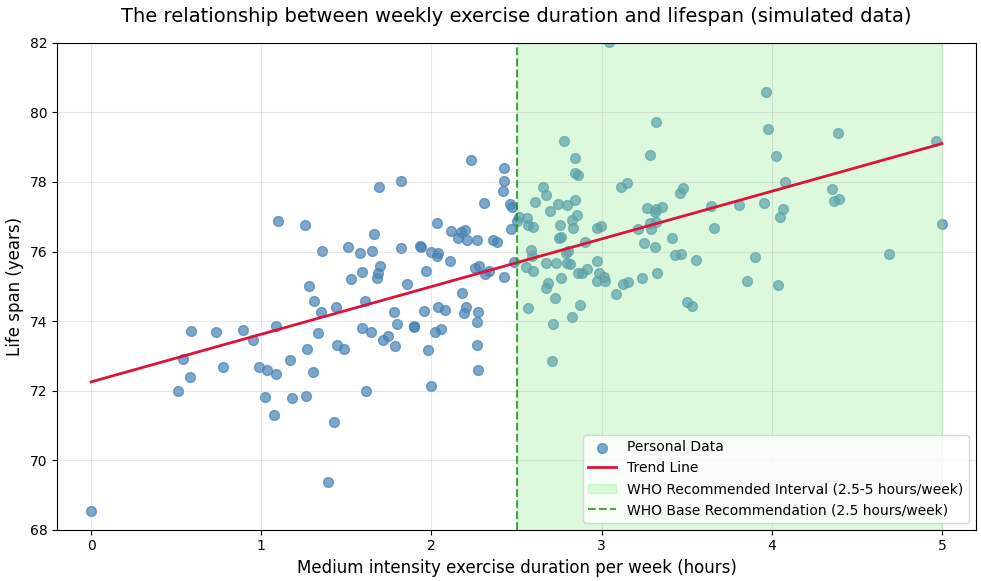
我们从一个简单的问题切入:每周运动时间和预期寿命的关系。
假设我们跟踪统计了200个人的每周运动时长和最终寿命,把数据画成散点图:横轴为每周运动小时数,纵轴为寿命。
生成模拟数据的 Python 代码
# Generate Simulated Data Fitting WHO Standard

import numpy as np
import matplotlib.pyplot as plt

# Set random seed for reproducibility
np.random.seed(42)

plt.rcParams['axes.unicode_minus'] = False  # fix minus display issue

# == 1. Generate Simulated Data Fitting WHO Standard
n_people = 200      # 200 samples
max_exercise = 5    # WHO recommended upper limit for moderate intensity exercise: 5 hours/week (300 minutes)
mean_exercise = 2.5 # WHO base recommendation for moderate intensity exercise: 2.5 hours/week (150 minutes)

# Generate exercise duration data: normal distribution (mean 2.5, std 1), more realistic than uniform distribution
exercise_hours = np.random.normal(loc=mean_exercise, scale=1, size=n_people)
# Clip values to ensure they are within the valid range: 0 ≤ exercise_hours ≤ 5 hours
exercise_hours = np.clip(exercise_hours, 0, max_exercise)

# Generate lifespan data: base lifespan 70 years + decreasing marginal benefit of exercise + random noise
base_lifespan = 70  # base lifespan
# Exercise benefit: use square root function to implement "marginal benefit decreasing" (benefit decreases as exercise duration increases)
exercise_benefit = 8 * np.sqrt(exercise_hours / max_exercise)  # benefit of 5 hours of exercise is about 8 years
# Random noise: normal distribution (mean 0, std 1.5), to simulate individual variability
random_noise = np.random.normal(loc=0, scale=1.5, size=n_people)
lifespan = base_lifespan + exercise_benefit + random_noise

# == 2. Plot Scatter Plot with Trend Line
plt.figure(figsize=(10, 6))

# Plot scatter plot
plt.scatter(
    exercise_hours, lifespan,
    color='steelblue', alpha=0.7, s=50,
    label='Personal Data'
)

# Fit linear trend line
z = np.polyfit(exercise_hours, lifespan, 1)
p = np.poly1d(z)
# Generate smooth x-axis data for trend line, to make it more visually appealing
x_smooth = np.linspace(0, max_exercise, 100)
plt.plot(
    x_smooth, p(x_smooth),
    color='crimson', linewidth=2,
    label='Trend Line'
)

# Annotate WHO recommended interval
plt.axvspan(2.5, 5, color='lightgreen', alpha=0.3, label='WHO Recommended Interval (2.5-5 hours/week)')
plt.axvline(x=2.5, color='forestgreen', linestyle='--', alpha=0.8, label='WHO Base Recommendation (2.5 hours/week)')

# == 3. Add Annotations
plt.title('The relationship between weekly exercise duration and lifespan (simulated data)', fontsize=14, pad=15)
plt.xlabel('Medium intensity exercise duration per week (hours)', fontsize=12)
plt.ylabel('Life span (years)', fontsize=12)
plt.xlim(-0.2, max_exercise + 0.2)  # x-axis range
plt.ylim(68, 82)  # y-axis range
plt.grid(True, alpha=0.3)
plt.legend(loc='lower right')

# Show plot
plt.tight_layout()
plt.savefig('exercise_hours_and_lifespan.png', dpi=150, bbox_inches='tight')
plt.show()
print("Image was saved as 'exercise_hours_and_lifespan.png'")

# Output core statistics
corr = np.corrcoef(exercise_hours, lifespan)[0, 1]
print(f'Correlation between weekly exercise duration and lifespan: {corr:.2f} (positive correlation, as expected)')
print(f'Average weekly exercise duration: {np.mean(exercise_hours):.1f} hours/week (close to WHO base recommendation of 2.5 hours)')
print(f'Average lifespan: {np.mean(lifespan):.1f} years')
世界卫生组织(WHO)推荐的成人每周运动时长为中等强度2.5~5小时,或高强度1.25~2.5小时,额外搭配2次力量训练(适用于18~64岁成年人)。
就如图中红线所示,我们会发现一个模糊但明显的趋势:运动时间越长的人,寿命大概率也越长。
线性回归要做的,就是在这些散点中,画一条最贴合的直线,这条直线代表了运动时长与寿命的关系。
这条直线的方程可以写成:
\[ \hat{y} := wx + b \]其中
- $\hat{y}$:预期寿命
- $x$:每周运动小时数
- $w$:权重系数(weight),代表运动时长对寿命的影响程度,值越大,说明运动对寿命的提升作用越明显
- $b$:截距项(bias),可以理解为基础寿命值,哪怕一个人完全不运动,也能拥有的寿命基数
$w$和$b$是线性回归模型要学习的参数,有了这两个参数值,就可以通过每周运动时长预测一个人的预期寿命。
这个方程就是一句大白话:基础寿命,加上运动带来的增益,就是预期寿命。
当影响因素变多,比如遗传、饮食、吸烟等,线性回归也能轻松应对,只需要为每个影响因素分配对应的权重参数,然后把它们的影响加起来就行,这就是多元线性回归。
多元线性回归模型#
参考《Nature》、《柳叶刀》等顶级期刊的研究结论,筛选出7个影响寿命的因素:
| 影响因素 | 英文名 | 数学变量 | 量化方式 |
|---|---|---|---|
| 父母平均寿命 | parent_lifespan | $x_1$ | 连续变量(岁),比如父母平均寿命75岁 |
| 性别 | gender | $x_2$ | 分类变量(0=男性,1=女性) |
| 每周中等强度运动时长 | exercise_hours | $x_3$ | 连续变量(小时),范围0~10小时 |
| 是否长期吸烟 | smoking | $x_4$ | 分类变量:0=不吸烟,1=长期吸烟 |
| 饮食健康程度 | diet_health | $x_5$ | 分类变量:0=高油高糖高盐,1=低脂低糖低盐 |
| 每日睡眠时长 | sleep_hours | $x_6$ | 连续变量(小时),范围5~9小时 |
| 压力/心理健康水平 | stress_level | $x_7$ | 分类变量:0=长期高压,1=压力适中,2=低压力/社交支持充足 |
上面的因素称为特征,是模型的自变量。
因为我们现在有了更多个因素,所以需要更多个权重系数,分别使用$w_1, w_2, w_3, w_4, w_5, w_6, w_7$来表示。
所以因变量为预期寿命(actual_lifespan):
\[ \hat{y} := w_1 x_1 + w_2 x_2 + w_3 x_3 + w_4 x_4 + w_5 x_5 + w_6 x_6 + w_7 x_7 + b \]$w_1, w_2, w_3, w_4, w_5, w_6, w_7, b$就是我们想求解的权重系数,也叫模型参数,由计算机利用训练数据自动学习得到
有了权重系数,知道了输入的自变量因素$\boldsymbol{x}$,就可以通过上式计算预测寿命了。
这就是线性回归模型的概念,接下来看一个完整的例子。